Numbers have an important story to tell. They rely on you to give them a voice - Alex Peiniger
Once you are done with your EDA and implemented a model, we need to evaluate how well a model has performed and this is done using multiple evaluation metrics. In this post, I will briefly explain how classification problems are different than regression problems. I will load the Mushroom Classification dataset, implement and explain multiple classification metrics such as, accuracy, precision and recall(sensitivity).

Regression VS Classification
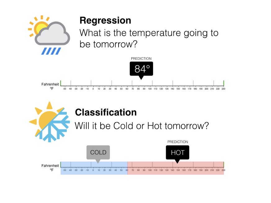
Machine Learning consists of many techniques to answer certain types of questions. These algorithms can be divided into the type of outputs they produce, that is, either continuous or discreate.
Regression models are used to predict continuous values. That is, the outputs of a regression models are not confined to a set of bins or labels. Predicting accumulated wealth based on age and education level.
On the other hand, classification models predict discrete values. That is, the predicted value is one of the possible outcomes in the finite set. A classification regression that predicts one of the two values is called binary classification. Predicting hotdog/not hotdog is an example of binary classification. In contrast, predicting one of multiple possible outcomes is called a multi-label classification. Customer segmentation is a good example of multi-label classification problem.

Now that we understand the difference between regression and classification problems, let's load the mushroom classification dataset, use mapper to convert strings into numbers for the models, fit the easiest classification model aka, decision trees and finally score it on different metrics. NOTE: Mushroom dataset is binary classification problem as we have to predict whether the mushroom is poisonous or edible. Let's get started!
Reading the Dataset below
import pandas as pd
df = pd.read_csv('mushrooms.csv')
df.head(3)
| class | cap-shape | cap-surface | cap-color | bruises | odor | gill-attachment | gill-spacing | gill-size | gill-color | ... | stalk-surface-below-ring | stalk-color-above-ring | stalk-color-below-ring | veil-type | veil-color | ring-number | ring-type | spore-print-color | population | habitat | |
|---|---|---|---|---|---|---|---|---|---|---|---|---|---|---|---|---|---|---|---|---|---|
| 0 | p | x | s | n | t | p | f | c | n | k | ... | s | w | w | p | w | o | p | k | s | u |
| 1 | e | x | s | y | t | a | f | c | b | k | ... | s | w | w | p | w | o | p | n | n | g |
| 2 | e | b | s | w | t | l | f | c | b | n | ... | s | w | w | p | w | o | p | n | n | m |
3 rows × 23 columns
Train_Test_Split the data as it is good practice and one should do it, if possible.
from sklearn.model_selection import train_test_split
y = df['class']

X = df.drop(['class','cap-color','bruises','odor','ring-number','gill-attachment','gill-spacing','gill-size','gill-color'], axis = 1)
X_train, X_test, y_train, y_test = train_test_split(X,y, random_state = 42)
In the following block of code, I have used data frame mapper, categorical imputer, label binarizer and pipeline to transform and fit the data to evaluate the model on different classification metrics. The main point of this post is to explain the classification metrics rather than transforming the data, therefore, you can skip the following piece of code.
from sklearn_pandas import DataFrameMapper, CategoricalImputer
from sklearn.preprocessing import LabelBinarizer
from sklearn.metrics import confusion_matrix
from sklearn.pipeline import make_pipeline
from sklearn.linear_model import LogisticRegression


#Scalling/Transforming our Features
mapper = DataFrameMapper([
('cap-shape',[CategoricalImputer(),LabelBinarizer()]),
('cap-surface',[CategoricalImputer(),LabelBinarizer()]),
('stalk-shape',[CategoricalImputer(),LabelBinarizer()]),
('stalk-root',[CategoricalImputer(),LabelBinarizer()]),
('stalk-surface-above-ring',[CategoricalImputer(),LabelBinarizer()]),
('stalk-surface-below-ring',[CategoricalImputer(),LabelBinarizer()]),
('stalk-color-above-ring',[CategoricalImputer(),LabelBinarizer()]),
('stalk-color-below-ring',[CategoricalImputer(),LabelBinarizer()]),
('veil-type',[CategoricalImputer(),LabelBinarizer()]),
('veil-color',[CategoricalImputer(),LabelBinarizer()]),
('ring-type',[CategoricalImputer(),LabelBinarizer()]),
('spore-print-color',[CategoricalImputer(),LabelBinarizer()]),
('population',[CategoricalImputer(),LabelBinarizer()]),
('habitat',[CategoricalImputer(),LabelBinarizer()]),
#('cap-color',[CategoricalImputer(),LabelBinarizer()]),
#('bruises',[CategoricalImputer(),LabelBinarizer()]),
#('odor',[CategoricalImputer(),LabelBinarizer()]),
#('gill-attachment',[CategoricalImputer(),LabelBinarizer()]),
#('gill-spacing',[CategoricalImputer(),LabelBinarizer()]),
#('gill-size',[CategoricalImputer(),LabelBinarizer()]),
#('gill-color',[CategoricalImputer(),LabelBinarizer()]),
#('ring-number',[CategoricalImputer(),LabelBinarizer()]),
],df_out = True)

#Pipeline to instantiate the mapper and decision tree classifier.
pipe = make_pipeline(
    mapper,
    LogisticRegression(solver='lbfgs',max_iter=200)
)
#Fitting our models
pipe.fit(X_train,y_train)
#Creating predictions
predicted = pipe.predict(X_test);
Just to sum up, I implemented logistic regression in the above code and predicted values for my X_test dataset. I dropped some columns from my X_train and X_test just so that I can get more discrepancy.

Confusion Matrix
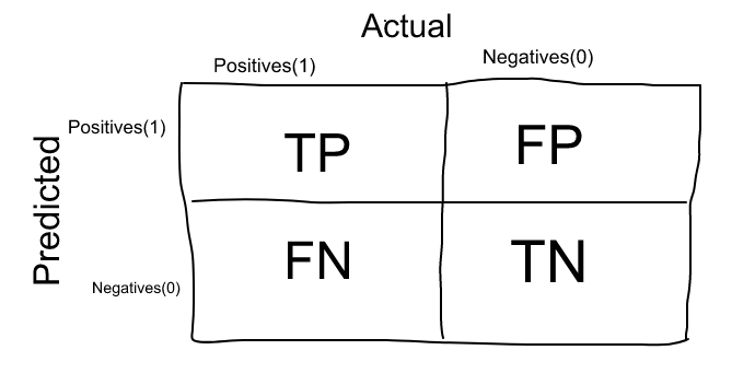
Confusion Matrix is not an evaluation model, however it can be used to find correctness and accuracy of a model. In addition, most of the classification metrics are based on the terms and numbers evaluated by it. Therefore, I will implement confusion matrix and then try to explain the terms associated with it.
Note: For this example, 1 represents my positive condition that is, that the mushroom is poisonous and 0 represents my negative condition that is, the mushroom is edible. Seems weird but think in terms of disease
cm = confusion_matrix(y_test,predicted)
cm_df = pd.DataFrame(data=cm, columns=['predicted poisonous', 'predicted edible'], index=['actual poisonous', 'actual edible'])
cm_df
| predicted poisonous | predicted edible | |
|---|---|---|
| actual poisonous | 1013 | 27 |
| actual edible | 5 | 986 |
To begin with, the baseline to read a confusion matrix starts by reading the diagonal from top-left to bottom-right. These two values,1013 and 986, in the above data frame are the correctly predicted values.
True Positive(TP) values are the cases when the positive condition is predicted correctly. We could also say that the model predicted 1 and the actual value was also 1. In this example, 1013 is the True Positive value, representing the correctly predicted poisonous mushroom.
True Negatives(TN) values are the cases when negative condition is correctly predicted. In other words, the model predicted 0 and the actual value was also 0. In this example 986 is the True Negative value, as it represents correctly edible poisonous mushrooms.
Now that we analyzed diagonal from top-left to bottom-right, let's look at the other diagonal. The other two values, that is 27 and 5 are called False Positive and False Negative, respectively. These terms are probably what adds confusion in the confusion matrix, so let's go.
False Positive(FP) values are the cases when positive condition is NOT predicted correctly. That is, the model predicted 0 and the actual value was 1. In our example, 27 is the False Positive value, representing poisonous mushrooms that were predicted to be edible.
False Negatives(TN) values are the cases when negative condition is NOT correctly predicted. In other words, the model predicted 1 and the actual value was also 0. In this example, 5 is the False Negative value, as it represents edible mushrooms that were deemed poisonous.

Now that we sort-off understand the four terms, we can use them create multiple classification metrics such as accuracy, precision, recall and f1-score.
Accuracy
To begin with, accuracy accounts for the overall performance of the model. We could also say that it is a ratio of correctly predicted observations to the total observations. The formula for accuracy is following:
Intuitively, accuracy seems to be logical and one would think about just using this as a evaluation tool of the model. However, accuracy score falls short when there are unbalanced classes. In other words, accuracy is not reliable when there are more TP over TN or vice versa. For instance, if you have 100 credit transactions and out of those you have 5 credit fraud cases. If our model only predicts no fraud cases, our model would be 95% accurate. Therefore, accuracy should not be used when the target variables are not balanced. We calculated using the formula, now let us see how was can implement accuracy_score and get similar if not exact same score:
from sklearn.metrics import accuracy_score
ac = accuracy_score(predicted,y_test)
ac
0.9842442146725751
Precision
Precision on the other hand, only calculates how accurate the predictions regarding the positive case are(poisonous mushrooms are positive case in our example).Precision is calculated by taking the ratio of correctly predicted positive observations to the total predicted positive observations. The formula for precision is following:
All in all, precision gives us the number in terms of our positive case. In the mushroom example, we are worried about the FP as marking an poisonous mushroom edible is harmful or deadly. Let us implement precision using sklearn.
Remember: High precision relates to the low false positive rate.
from sklearn.metrics import precision_score
pc = precision_score(y_test,predicted, average='weighted')
pc
0.9844797253017756
Recall
Recall also know as sensitivity is a score for the coverage of actual positive sample. Recall is calculated by taking the ratio of correctly predicted positive cases to the all cases are in actual class. Let's look at the formula as it helped me understand the concept so it might help you too!
For our example, recall score would judge how well our model predicted positive cases when the actual case was positive. There is a trade-off between precision and recall score. Which evaluation metrics you use, depends on each problem.
Note: Specificity is another classification metrics that is the opposite of Recall.
Let's us implement recall from sklearn.
from sklearn.metrics import recall_score
rc = recall_score(y_test, predicted, average='weighted')
rc
0.9842442146725751
All in all, all these terms can be used to get understand another classification metrics, F1-Score. But I guess the blog is already too long, so let's keep that for another day.