According to the official site for scikit-image, "scikit-image is a collection of algorithms for image processing". As I learning about image processing, I seem to find more tutorials for OpenCV and Pillow rather than scikit-image, even though it comes pre-installed with several Python distributions. So here is my quick tutorial that might help you get started.
I will present basic operations, such as reading multiple pictures, converting them to gray scale, resizing and transforming the pictures as I work towards my image classification problem. I am following same format as Pillow's blog so that you can compare the two image processing libraries for yourself.
Loading the Image
Let's get started. We first load the image, using the imread routine from scikit-image.
import os
import numpy as np
import random
import re
from sklearn.preprocessing import MinMaxScaler

from skimage.io import imshow,imread,imsave, ImageCollection
from skimage.color import rgb2gray
from skimage.transform import rescale, resize, rotate
from skimage.util import random_noise

import warnings
warnings.filterwarnings(action='ignore', category=UserWarning)

import matplotlib.pyplot as plt
Now that we have imported io from skimage, we can use absolute path to read a file. Scikit image's package, imread, is used to read an image as an array. YES, you read it correct, AS AN ARRAY. You might be wondering, why is this exciting? This means we manipulate the picture using other libraries in the Python Ecosystem, such as matplotlib and scipy. For example, you can see in the code below, you will see that the images are being displayed using the matplotlib.
directory = 'C:/Users/m_mas/Desktop/skit-image/'
img = imread(directory +'img_processing1.JPG')
grayscale = rgb2gray(img)
fig, axes = plt.subplots(figsize=(10,10),nrows=1, ncols=2)

ax = axes.ravel()

ax[0].imshow(img)
ax[0].set_title("Original image")

ax[1].imshow(grayscale, cmap = 'gray')
ax[1].set_title("GrayScale")


ax[0].set_xlim(0, 550)
ax[0].set_ylim(550,0)
plt.tight_layout(pad = 1)
plt.show();

print("Original Shape: "+ str(img.shape))
print("Gray Scaled Shape: "+ str(grayscale.shape))
Original Shape: (492, 538, 3)
Gray Scaled Shape: (492, 538)
Different Types and their meanings
The shape of the images tells us a lot. The third value in the shape of the original image indicates that the picture is a colored image rather than a gray scale. See below the table below for more combinations of shape you might encounter.
| Image Types | Coordinates |
|---|---|
| 2D Grayscale | (row,columns) |
| 2D Multichannel | (row,columns,channel) |
| 3D Grayscale | (plane, row,columns) |
| 3D Multichannel | (plane,row,columns,channel) |
Data Augmentation - Trick to multiplying your data
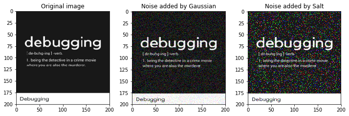
To perform well on an image classifier you would need a lot of images to train. Web scrapping will get you started however you can drastically change the performance of your classifier by making an exhaustive dataset. Image data augmentation can be used to expand the size of our dataset by creating modified versions of the images in the existing dataset. You can scale(rescale/resize), flip(flipud/flipur), rotate or adding gaussian noise to get more of your limited dataset.

Rescalling and Resizing
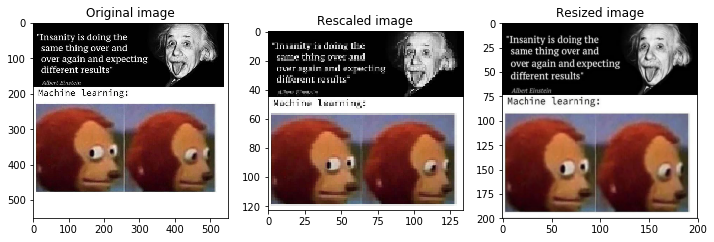
Rescaling and resizing are helpful tools that could be used for processing images. Rescaling shrinks an image by a given factor. In the example before, the scaling factor is 0.25 and the image size of 492 X 538 will be reduced to 142 X125. The scaling factor can be a either a floating point or a tuple containing value for each axis.
On a similar note, resizing let's you specify the shape of the image. In the example below our original image (492, 538) with be shaped to 200 X 200 pixels.
image_rescaled = rescale(img, 0.25, anti_aliasing=False)
print("Shape after rescalling : "+str(image_rescaled.shape))
image_resized = resize(img,(200,200),anti_aliasing=True)
# print("Shape after resizing : "+str(image_resized.shape))

fig, axes = plt.subplots(figsize=(10,10),nrows=1, ncols=3)

ax = axes.ravel()

ax[0].imshow(img)
ax[0].set_title("Original image")

ax[1].imshow(image_rescaled)
ax[1].set_title("Rescaled image")

ax[2].imshow(image_resized)
ax[2].set_title("Resized image")

ax[0].set_xlim(0, 550)
ax[0].set_ylim(550,0)
plt.tight_layout(pad = 1)
plt.show();
Shape after rescalling : (123, 134, 3)
Transforming / Altering the images
Flipping Images
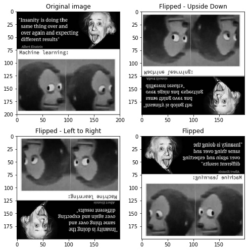
As the images are imported as an array, you can use numpy methods to flip images horizontally(fliplr) and vertically(flipud). However in the code below, I flipped the horizontally flipped image vertically to get a third type of flip. Too wordy right? Try to understand the code below, and I am sure you would get it.
image_resized = resize(img,(200,200), anti_aliasing=True)

# Image tansformations
img = rgb2gray(image_resized)
ud_img = rgb2gray(np.flipud(img))
lr_img = rgb2gray(np.fliplr(ud_img))
fourth_img = rgb2gray(np.flipud(lr_img))

#The above code is just for plotting the images
fig, axes = plt.subplots(figsize=(7,7),nrows=2, ncols=2)

ax = axes.ravel()

ax[0].imshow(img, cmap = 'gray')
ax[0].set_title("Original image")

ax[1].imshow(ud_img, cmap = 'gray')
ax[1].set_title("Flipped - Upside Down")

ax[2].imshow(lr_img, cmap = 'gray')
ax[2].set_title("Flipped - Left to Right")

ax[3].imshow(fourth_img, cmap = 'gray')
ax[3].set_title("Flipped")

ax[0].set_xlim(0, 200)
ax[0].set_ylim(200,0)
plt.tight_layout(pad = 1)
plt.show()
Rotating with Random integer
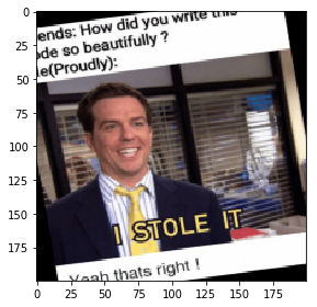
In the code below, we will be randomly generating a number between -40 and 40 and then will be using the number to rotate the image.
img = imread(directory +'img_processing3.png')
rand_dregree = random.uniform(-40,40)
rotated = rotate(img, rand_dregree)
rotated = resize(rotated,(200,200),anti_aliasing=True)
imshow(rotated)
<matplotlib.image.AxesImage at 0x1d79dea02e8>
img = imread(directory +'img_processing4.png')

img = resize(img,(200,200),anti_aliasing=True)

gaussian_img = random_noise(img, mode = 'gaussian')
salt_img = random_noise(img, mode = 'salt')

fig, axes = plt.subplots(figsize=(10,10),nrows=1, ncols=3)

ax = axes.ravel()

ax[0].imshow(img)
ax[0].set_title("Original image")

ax[1].imshow(gaussian_img)
ax[1].set_title("Noise added by Gaussian")

ax[2].imshow(salt_img)
ax[2].set_title("Noise added by Salt")

ax[0].set_xlim(0, 200)
ax[0].set_ylim(200,0)
plt.tight_layout(pad = 1)
plt.show();
Saving the transformed images
You can import imsave from io to save the new files on your computer. Imsave saves the new file on the same file level from where you are running the script. This method use two parameters, new file name as fname and the file you want to save as arr. 'fname' also let's you change the format of the file. For instance, you can save a jpg file as png file or vice versa just by changing the name of the file.
Note: The picture imported below is a jpg and we would change the format to png.
img = imread(directory +'img_processing4.png')
output_directory = directory + 'editted'+'/'
imsave(output_directory+'edit.png', img)
Making Changes to all the pictures
You can certainly make a loop to get the name of the files and load then to make the changes. However, Scikit-image provides your a feature called Image Collection that let's you load all the images in the memory in one go. Image Collection takes a wild card as it's parameters. To begin with, let me show you a simple for loop to load the images and then I can show you how image collection can do the same job in one line.
For Loop to load the images.
files = []

def get_files(directory):
    for file in os.listdir(directory):
        if file.startswith("img_"):
            files.append(file)
    return files

files_name = get_files(directory)
files_name
['img_processing1.JPG',
 'img_processing2.jpg',
 'img_processing3.png',
 'img_processing4.png']
Image Collection to load the images.
ic = ImageCollection('C:/Users/m_mas/Desktop/skit-image/*.*')
ic.files
['C:/Users/m_mas/Desktop/skit-image\\img_processing1.JPG',
 'C:/Users/m_mas/Desktop/skit-image\\img_processing2.jpg',
 'C:/Users/m_mas/Desktop/skit-image\\img_processing3.png',
 'C:/Users/m_mas/Desktop/skit-image\\img_processing4.png']
In the code below, I will be using all the transformation I used above and implement all of them on the four images I had in my folder. I will be changing the images in my folder to gray scale, adding random noise, rotating them by a certain degree and flipping them. All in all, I started with a dataset of 4 pictures and ended with 24 images that can be fed to a machine learning algorithm.
#Changes all of then to gray scale
scaler = MinMaxScaler(feature_range=(-0.99,0.99))

for files in files_name:
    file = re.findall(r'[a-z]+_[a-z]+\d',files)[0]

    #Reads a files
    temp_img = imread(directory + files)

    #Changes to gray scale and resizes the image to 200*200
    temp_gray = rgb2gray(temp_img)
    img = (resize(temp_gray,(200,200),anti_aliasing=True))
    img = scaler.fit_transform(img)
    imsave(output_directory+file+'1.jpg', img)

    #Random Noise
    salt_noise = random_noise(img, mode = 'salt')
    salt_img = scaler.fit_transform(salt_noise)
    imsave(output_directory+file+'2.jpg', salt_img)

    #Rotating the image and saving the file
    rand_dregree = random.uniform(-25,25)
    temp_rotate = rotate(img, rand_dregree)
    imsave(output_directory+file+'3.png', temp_rotate)

    #Flipud - Veritcal Flip
    vert_flip = np.flipud(img)
    imsave(output_directory+file+'4.png', vert_flip)

    #Flipur - Horizontal Flip
    hori_flip = np.fliplr(vert_flip)
    imsave(output_directory+file+'5.png', hori_flip)

    #Flipud - Vertically Flipping the hoziontally flipped image
    vert_hori_flip = np.flipud(hori_flip)
    imsave(output_directory+file+'6.png', vert_hori_flip)
All in all, Scikit image is good package to start data augmentation to expand your dataset. You can surely use different combinations to increase your dataset even more. For instance, add different type of noise on a rotated images.
